Python支持向量机非线性回归(SVR)模型实战:核函数参数调优详解

发布时间:2026-10-13 |
2人浏览过
本文深入解析Python中支持向量机(SVR)在非线性回归任务中的应用。通过scikit-learn库加载糖尿病数据集,系统演示了线性、多项式、高斯(RBF)及Sigmoid四种核函数的实现方法。重点探讨多项式阶数、正则化系数及gamma值对模型训练得分与测试得分的影响,提供可视化分析代码,帮助开发者理解不同核函数及超参数对SVR预测性能的具体影响,适用于机器学习入门及模型调优参考。
SVR模型基础与数据加载
本文详细讲解基于Python的支持向量机(SVR)非线性回归模型构建过程。为便于读者直接上手,下文将逐步展开代码实现与原理分析。
线性核SVR实现
import numpy as np
import matplotlib.pyplot as plt

from sklearn import datasets, linear_model,svm
from sklearn.model_selection import train_test_split

def load_data_regression():
  '''
  加载用于回归问题的数据集
  '''
  diabetes = datasets.load_diabetes() #使用 scikit-learn 自带的一个糖尿病病人的数据集
  # 拆分成训练集和测试集,测试集大小为原始数据集大小的 1/4
  return train_test_split(diabetes.data,diabetes.target,test_size=0.25,random_state=0)

#支持向量机非线性回归SVR模型
def test_SVR_linear(*data):
  X_train,X_test,y_train,y_test=data
  regr=svm.SVR(kernel='linear')
  regr.fit(X_train,y_train)
  print('Coefficients:%s, intercept %s'%(regr.coef_,regr.intercept_))
  print('Score: %.2f' % regr.score(X_test, y_test))

# 生成用于回归问题的数据集
X_train,X_test,y_train,y_test=load_data_regression()
# 调用 test_LinearSVR
test_SVR_linear(X_train,X_test,y_train,y_test)
多项式核参数影响分析
def test_SVR_poly(*data):
  '''
  测试 多项式核的 SVR 的预测性能随 degree、gamma、coef0 的影响.
  '''
  X_train,X_test,y_train,y_test=data
  fig=plt.figure()
  ### 测试 degree ####
  degrees=range(1,20)
  train_scores=[]
  test_scores=[]
  for degree in degrees:
    regr=svm.SVR(kernel='poly',degree=degree,coef0=1)
    regr.fit(X_train,y_train)
    train_scores.append(regr.score(X_train,y_train))
    test_scores.append(regr.score(X_test, y_test))
  ax=fig.add_subplot(1,3,1)
  ax.plot(degrees,train_scores,label="Training score ",marker='+' )
  ax.plot(degrees,test_scores,label= " Testing score ",marker='o' )
  ax.set_title( "SVR_poly_degree r=1")
  ax.set_xlabel("p")
  ax.set_ylabel("score")
  ax.set_ylim(-1,1.)
  ax.legend(loc="best",framealpha=0.5)

  ### 测试 gamma,固定 degree为3, coef0 为 1 ####
  gammas=range(1,40)
  train_scores=[]
  test_scores=[]
  for gamma in gammas:
    regr=svm.SVR(kernel='poly',gamma=gamma,degree=3,coef0=1)
    regr.fit(X_train,y_train)
    train_scores.append(regr.score(X_train,y_train))
    test_scores.append(regr.score(X_test, y_test))
  ax=fig.add_subplot(1,3,2)
  ax.plot(gammas,train_scores,label="Training score ",marker='+' )
  ax.plot(gammas,test_scores,label= " Testing score ",marker='o' )
  ax.set_title( "SVR_poly_gamma r=1")
  ax.set_xlabel(r"$\gamma$")
  ax.set_ylabel("score")
  ax.set_ylim(-1,1)
  ax.legend(loc="best",framealpha=0.5)
  ### 测试 r,固定 gamma 为 20,degree为 3 ######
  rs=range(0,20)
  train_scores=[]
  test_scores=[]
  for r in rs:
    regr=svm.SVR(kernel='poly',gamma=20,degree=3,coef0=r)
    regr.fit(X_train,y_train)
    train_scores.append(regr.score(X_train,y_train))
    test_scores.append(regr.score(X_test, y_test))
  ax=fig.add_subplot(1,3,3)
  ax.plot(rs,train_scores,label="Training score ",marker='+' )
  ax.plot(rs,test_scores,label= " Testing score ",marker='o' )
  ax.set_title( "SVR_poly_r gamma=20 degree=3")
  ax.set_xlabel(r"r")
  ax.set_ylabel("score")
  ax.set_ylim(-1,1.)
  ax.legend(loc="best",framealpha=0.5)
  plt.show()

# 调用 test_SVR_poly
test_SVR_poly(X_train,X_test,y_train,y_test)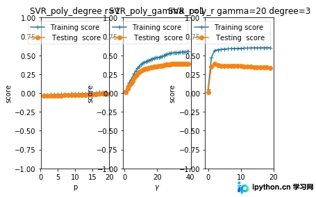
高斯核(RBF)参数调优
def test_SVR_rbf(*data):
  '''
  测试 高斯核的 SVR 的预测性能随 gamma 参数的影响
  '''
  X_train,X_test,y_train,y_test=data
  gammas=range(1,20)
  train_scores=[]
  test_scores=[]
  for gamma in gammas:
    regr=svm.SVR(kernel='rbf',gamma=gamma)
    regr.fit(X_train,y_train)
    train_scores.append(regr.score(X_train,y_train))
    test_scores.append(regr.score(X_test, y_test))
  fig=plt.figure()
  ax=fig.add_subplot(1,1,1)
  ax.plot(gammas,train_scores,label="Training score ",marker='+' )
  ax.plot(gammas,test_scores,label= " Testing score ",marker='o' )
  ax.set_title( "SVR_rbf")
  ax.set_xlabel(r"$\gamma$")
  ax.set_ylabel("score")
  ax.set_ylim(-1,1)
  ax.legend(loc="best",framealpha=0.5)
  plt.show()

# 调用 test_SVR_rbf
test_SVR_rbf(X_train,X_test,y_train,y_test)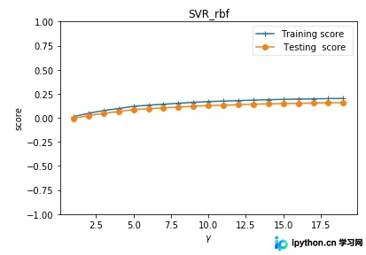
Sigmoid核性能测试
def test_SVR_sigmoid(*data):
  '''
  测试 sigmoid 核的 SVR 的预测性能随 gamma、coef0 的影响.
  '''
  X_train,X_test,y_train,y_test=data
  fig=plt.figure()

  ### 测试 gammam,固定 coef0 为 0.01 ####
  gammas=np.logspace(-1,3)
  train_scores=[]
  test_scores=[]

  for gamma in gammas:
    regr=svm.SVR(kernel='sigmoid',gamma=gamma,coef0=0.01)
    regr.fit(X_train,y_train)
    train_scores.append(regr.score(X_train,y_train))
    test_scores.append(regr.score(X_test, y_test))
  ax=fig.add_subplot(1,2,1)
  ax.plot(gammas,train_scores,label="Training score ",marker='+' )
  ax.plot(gammas,test_scores,label= " Testing score ",marker='o' )
  ax.set_title( "SVR_sigmoid_gamma r=0.01")
  ax.set_xscale("log")
  ax.set_xlabel(r"$\gamma$")
  ax.set_ylabel("score")
  ax.set_ylim(-1,1)
  ax.legend(loc="best",framealpha=0.5)
  ### 测试 r ,固定 gamma 为 10 ######
  rs=np.linspace(0,5)
  train_scores=[]
  test_scores=[]

  for r in rs:
    regr=svm.SVR(kernel='sigmoid',coef0=r,gamma=10)
    regr.fit(X_train,y_train)
    train_scores.append(regr.score(X_train,y_train))
    test_scores.append(regr.score(X_test, y_test))
  ax=fig.add_subplot(1,2,2)
  ax.plot(rs,train_scores,label="Training score ",marker='+' )
  ax.plot(rs,test_scores,label= " Testing score ",marker='o' )
  ax.set_title( "SVR_sigmoid_r gamma=10")
  ax.set_xlabel(r"r")
  ax.set_ylabel("score")
  ax.set_ylim(-1,1)
  ax.legend(loc="best",framealpha=0.5)
  plt.show()

# 调用 test_SVR_sigmoid
test_SVR_sigmoid(X_train,X_test,y_train,y_test)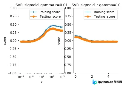
总结
以上内容涵盖了SVR模型的核心实现与参数测试方法,希望能为读者的机器学习实践提供有益参考。欢迎持续关注本站获取更多技术资源。
本站声明
本文内容仅供参考,不代表本站观点。转载或引用请注明出处。如发现内容问题,请通过联系我们页面反馈。