Python实现Logistic回归分类算法：从原理到代码

山间有风

发布时间：2026-10-13 | 2人浏览过

原创

本文基于吴恩达机器学习课程，使用Python实现了Logistic分类算法。详细阐述了如何通过Sigmoid函数将线性回归输出映射至0-1区间，并定义了代价函数。通过梯度下降法迭代优化参数theta，最终给出完整的Python实现代码及运行结果，帮助读者理解二分类问题的数学原理与编程实践。

Logistic回归算法实现概述

近期在研读吴恩达的机器学习课程时，笔者尝试使用Python复现了其中的Logistic算法，并利用梯度下降法求解最优参数。

Logistic分类主要解决二分类问题。对于线性回归函数，其输出值域为负无穷到正无穷，这并不直接适用于分类任务。

假设函数与分类边界

在分类问题中，我们希望假设函数的输出值落在0到1之间。因此，需要对Logistic函数的假设函数进行变换处理。

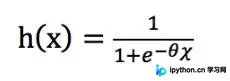
从上述公式可以看出，变换后的h(x)取值范围在0到1之间。基于此，我们可以设定1/2作为分类的分界线。

代价函数与梯度下降优化

代价函数（Cost Function）的定义方式如下。

其中，m代表样本数量。初始阶段，theta可以随机赋予一个初始值，计算出初始的J(theta)值，随后执行梯度下降算法进行迭代，直至逼近最优值。迭代的核心在于每次减去一个偏导量。

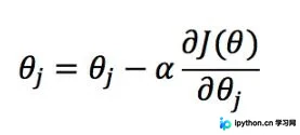
将J(theta)代入公式化简后，可以发现其迭代函数形式与线性回归中的迭代函数相同。

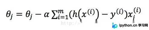
依据该迭代函数不断调整theta的值，当两次计算的J(theta)值之差小于某个极小阈值时，即可认为达到了最优解。需要注意的是，这通常是一个相对较优的解，而非绝对全局最优解。其中，alpha为学习速率；学习速率越大，收敛速度越快，但若设置过大可能导致代价函数无法收敛。完整的Python实现代码如下。

Python代码实现与测试


import math

ALPHA = 0.3
DIFF = 0.00001


def predict(theta, data):
  results = []
  for i in range(0, data.__len__()):
    temp = 0
    for j in range(1, theta.__len__()):
      temp += theta[j] * data[i][j - 1]
    temp = 1 / (1 + math.e ** (-1 * (temp + theta[0])))
    results.append(temp)
  return results


def training(training_data):
  size = training_data.__len__()
  dimension = training_data[0].__len__()
  hxs = []
  theta = []
  for i in range(0, dimension):
    theta.append(1)
  initial = 0
  for i in range(0, size):
    hx = theta[0]
    for j in range(1, dimension):
      hx += theta[j] * training_data[i][j]
    hx = 1 / (1 + math.e ** (-1 * hx))
    hxs.append(hx)
    initial += (-1 * (training_data[i][0] * math.log(hx) + (1 - training_data[i][0]) * math.log(1 - hx)))
  initial /= size
  iteration = initial
  initial = 0
  counts = 1
  while abs(iteration - initial) > DIFF:
    print("第", counts, "次迭代, diff=", abs(iteration - initial))
    initial = iteration
    gap = 0
    for j in range(0, size):
      gap += (hxs[j] - training_data[j][0])
    theta[0] = theta[0] - ALPHA * gap / size
    for i in range(1, dimension):
      gap = 0
      for j in range(0, size):
        gap += (hxs[j] - training_data[j][0]) * training_data[j][i]
      theta[i] = theta[i] - ALPHA * gap / size
      for m in range(0, size):
        hx = theta[0]
        for j in range(1, dimension):
          hx += theta[j] * training_data[i][j]
        hx = 1 / (1 + math.e ** (-1 * hx))
        hxs[i] = hx
        iteration += -1 * (training_data[i][0] * math.log(hx) + (1 - training_data[i][0]) * math.log(1 - hx))
      iteration /= size
    counts += 1
  print('training done,theta=', theta)
  return theta


if __name__ == '__main__':
  training_data = [[1, 1, 1, 1, 0, 0], [1, 1, 0, 1, 0, 0], [1, 0, 1, 0, 0, 0], [0, 0, 0, 0, 1, 1], [0, 1, 0, 0, 0, 1],
        [0, 0, 0, 0, 1, 1]]
  test_data = [[0, 1, 0, 0, 0], [0, 0, 0, 0, 1]]
  theta = training(training_data)
  res = predict(theta, test_data)
  print(res)

程序运行结果如下所示。