Python实现梯度下降法求解线性回归参数

发布时间:2026-10-13 |
5人浏览过
本文通过Python代码演示如何使用梯度下降法求解线性方程y=a*x1+b*x2+c中的最优参数a、b、c。基于给定的训练数据和测试数据,通过迭代更新参数,展示模型如何逐渐逼近真实值,为监督学习中的参数优化提供具体实现参考。
Python梯度下降法实现概述
本文分享了使用Python实现梯度下降法的具体代码,供读者参考学习。
开发工具为Python(x,y)2.6.6,运行环境为Windows10系统。
核心问题是求解线性方程y=2*x1+x2+3,即利用梯度下降法寻找参数a、b、c的最优值,这属于监督学习的范畴。
训练数据集如下:
x_train包含以下样本:[1, 2], [2, 1], [2, 3], [3, 5], [1, 3], [4, 2], [7, 3], [4, 5], [11, 3], [8, 7]。
对应的y_train标签值为:[7, 8, 10, 14, 8, 13, 20, 16, 28, 26]。
测试数据集如下:
x_test包含以下样本:[1, 4], [2, 2], [2, 5], [5, 3], [1, 5], [4, 1]。
梯度下降法核心代码解析
# -*- coding: utf-8 -*-
"""
Created on Wed Nov 16 09:37:03 2016
@author: Jason
"""

import numpy as np
import matplotlib.pyplot as plt

# y=2 * (x1) + (x2) + 3

rate = 0.001
x_train = np.array([[1, 2], [2, 1],[2, 3], [3, 5], [1, 3], [4, 2], [7, 3], [4, 5], [11, 3], [8, 7] ])
y_train = np.array([7, 8, 10, 14, 8, 13, 20, 16, 28, 26])
x_test = np.array([[1, 4],[2, 2],[2, 5],[5, 3],[1, 5],[4, 1]])

a = np.random.normal()
b = np.random.normal()
c = np.random.normal()

def h(x):
 return a*x[0]+b*x[1]+c

for i in range(100):
 sum_a=0
 sum_b=0
 sum_c=0

 for x, y in zip(x_train, y_train):
  for xi in x:
   sum_a = sum_a+ rate*(y-h(x))*xi
   sum_b = sum_b+ rate*(y-h(x))*xi
   #sum_c = sum_c + rate*(y-h(x)) *1

   a = a + sum_a
   b = b + sum_b
   c = c + sum_c
   plt.plot([h(xi) for xi in x_test])


print(a)
print(b)
print(c)

result=[h(xi) for xi in x_train]
print(result)

result=[h(xi) for xi in x_test]
print(result)

plt.show()
程序运行后的输出结果展示在下方图表中。
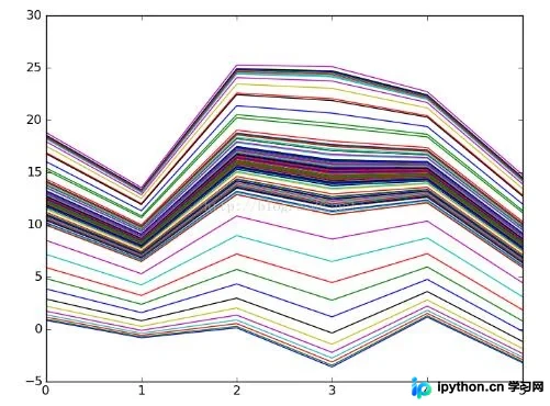
结论表明,随着迭代次数增加,预测线段逐渐逼近真实值;训练数据量越大,迭代次数越多,拟合效果越接近真实参数。
希望以上内容能对读者有所帮助,欢迎继续支持本站获取更多技术资源。
本站声明
本文内容仅供参考,不代表本站观点。转载或引用请注明出处。如发现内容问题,请通过联系我们页面反馈。