Python数据分析代码案例：Pandas清洗与Matplotlib可视化

Ada

发布时间：2026-11-11 | 2人浏览过

原创

本篇教程以真实的电商销售脏数据为例，详细演示如何使用Pandas进行缺失值填充、日期标准化、文本去噪与异常过滤，并通过Matplotlib面向对象接口绘制专业双轴统计图与趋势图。

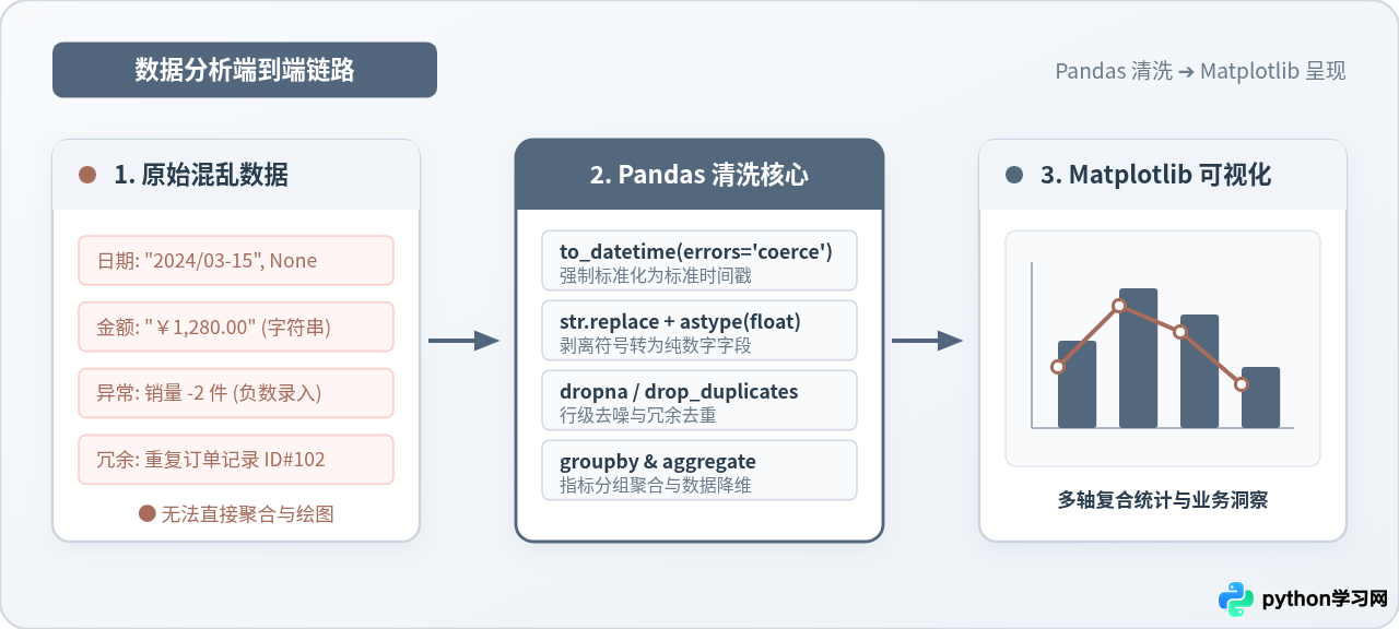
真实业务场景中的数据很少以整洁完备的状态直接呈现，往往混杂着格式混乱的日期、夹带货币符号的文本、缺失行及异常负值。本文通过一个典型的电商多渠道订单脏数据集，从零构建可执行的完整代码案例，演示如何运用 Pandas 实施系统化的数据清洗流，并借助 Matplotlib 面向对象机制输出具备专业出版水准的双轴统计图表。

Python数据分析代码案例：Pandas清洗与Matplotlib可视化 — 图 0：从混乱原始数据到 Pandas 清洗及 Matplotlib 结构化图表的全链路流程图

一、业务场景与脏数据集构建

很多数据分析教程往往依赖现成的标准化数据集（如鸢尾花数据集或小费数据集），这容易让初学者在面对真实业务环境时手足无措。在实际业务中，由于前端表单限制不严、多系统数据合并或人工手工录入，原始数据通常充满瑕疵。

为了还原最真实的清洗与分析过程，我们首先在 Python 中构造一个包含典型现实缺陷的销售订单表。该数据集包含订单号、下单时间、单价、购买数量与商品品类，共包含 10 条记录并埋伏了以下典型问题：

日期格式杂乱：混合了 "2024-03-01"、"2024/03/02"、中文格式 "2024年03月03日" 以及空值 None；
数值被存储为污染文本：单价列夹杂货币符号 ￥ 和千分位逗号 ,，导致 Pandas 将其识别为通用对象（object）类型；
主键重复：订单编号 1002 重复录入；
业务逻辑异常：存在购买数量为 -2 件的不合理脏记录；
维度缺失：部分记录的商品品类为 np.nan。

import pandas as pd
import numpy as np

# 构造包含典型缺陷的真实业务脏数据
raw_data = {
    'order_id': [1001, 1002, 1002, 1003, 1004, 1005, 1006, 1007, 1008, 1009],
    'order_date': [
        '2024-03-01', '2024/03/02', '2024/03/02', '2024年03月03日', None,
        '2024-03-04', '2024-03-05', '2024-03-05', '2024-03-06', '2024-03-07'
    ],
    'unit_price': [
        '￥1,200.00', '450.0', '450.0', '￥89.50', '￥3,200.00',
        '120.0', '￥2,100.00', '78.0', '￥560.00', '￥1,100.00'
    ],
    'quantity': [2, 1, 1, -2, 1, 3, 2, 5, 0, 2],
    'category': ['电子数码', '服饰鞋帽', '服饰鞋帽', '生鲜食品', '家居生活', None, '电子数码', '生鲜食品', '家居生活', '电子数码']
}

df = pd.DataFrame(raw_data)
print("--- 原始数据样本预览 ---")
print(df)

二、Pandas 数据缺陷探查与诊断

拿到任何陌生数据后，严禁直接开始计算指标或绘图。规范的流程是先进行三步基础诊断：类型核查、缺失统计和极值扫描。

运行 df.info() 可以发现，order_date 和 unit_price 均被标记为 object 类型。这代表 Pandas 将其视作普通字符串，此时不仅无法进行日期比较与重采样，也无法对单价执行加减乘除计算。同时，df.isnull().sum() 明确指出了日期与分类列均存在空值缺失。

排查要点：df.describe() 默认只针对数值列计算统计量。此时检查 quantity 列的最小值（min），会立刻暴露 -2 和 0 的异常值，这在真实商品购买中显然属于退款脏数据或无意义记录，必须在业务过滤阶段处理。

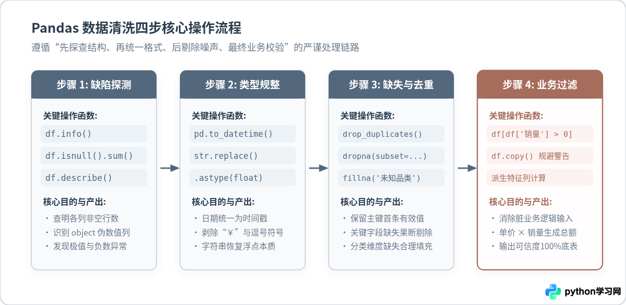
三、系统化数据清洗实操

根据诊断出的缺陷清单，我们按照标准化流程逐步执行清洗。每一步操作均采用矢量化方式进行，避免效率低下的 Python 原生循环。

1. 日期字段强制规整

面对混合斜杠、短横线与中文字符的日期字符串，直接使用 pd.to_datetime() 并搭配 errors='coerce' 参数。该参数的作用在于：一旦遇到无法解析的格式或非法字符，强制将其转化为 NaT（Not a Time），而不是抛出异常中断执行。

# 统一转换并处理非法日期
df['order_date'] = pd.to_datetime(
    df['order_date'].astype(str).str.replace('年', '-').str.replace('月', '-').str.replace('日', ''),
    errors='coerce'
)

2. 文本数值列的符号剥离与类型转换

单价字段中的 ￥ 和 , 是阻止数值转换的元凶。我们通过 Pandas 的字符串矢量接口 .str.replace() 剔除这些符号，随后通过 .astype(float) 转换恢复其浮点数本质：

# 清除货币符号与千分位逗号，转换为浮点型
df['unit_price'] = (
    df['unit_price']
    .str.replace('￥', '', regex=False)
    .str.replace(',', '', regex=False)
    .astype(float)
)

3. 重复值剔除与缺失值分类处理

业务中不同字段的缺失值处理策略截然不同：

主键重复：使用 df.drop_duplicates(subset=['order_id'], keep='first')，仅保留首条有效订单；
关键时间戳缺失：缺少日期的订单无法归入时间序列分析，属于关键字段缺失，直接调用 df.dropna(subset=['order_date']) 剔除整行；
属性维度缺失：商品品类虽有缺失，但订单金额真实存在，若直接删行会导致销售总额失真，因此使用 df['category'].fillna('其他品类') 进行填充归类。

4. 业务边界过滤与特征列派生

过滤掉销量小于等于 0 的脏记录后，务必调用 .copy() 方法生成独立副本，并重置行索引。随后计算派生字段 total_amount = unit_price * quantity：

# 剔除重复订单
df = df.drop_duplicates(subset=['order_id'], keep='first')

# 剔除日期缺失行，填充品类缺失值
df = df.dropna(subset=['order_date'])
df['category'] = df['category'].fillna('其他品类')

# 业务过滤：保留销售数量大于0的记录，使用 copy() 避免 SettingWithCopyWarning
clean_df = df[df['quantity'] > 0].copy()
clean_df.reset_index(drop=True, inplace=True)

# 派生特征：计算订单实际总金额
clean_df['total_amount'] = clean_df['unit_price'] * clean_df['quantity']
print("--- 清洗后的整洁数据表 ---")
print(clean_df[['order_id', 'order_date', 'category', 'unit_price', 'quantity', 'total_amount']])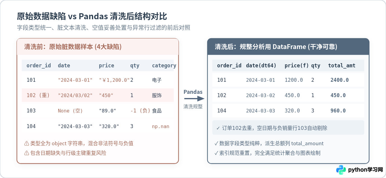

四、数据分组聚合计算

完成数据清洗后，底表结构清晰、数值纯正，可以直接进行统计聚合。为了满足后续多维图表的可视化需求，我们分别进行两个维度的聚合：

品类维度聚合：汇总各商品品类的销售总金额、总销售件数与平均客单价；
时间维度聚合：按日期汇总日销售额波动。

# 1. 品类维度聚合统计
category_summary = clean_df.groupby('category').agg(
    total_sales=('total_amount', 'sum'),
    total_quantity=('quantity', 'sum'),
    avg_price=('unit_price', 'mean')
).reset_index().sort_values(by='total_sales', ascending=False)

# 2. 日期维度趋势统计
daily_trend = clean_df.groupby('order_date').agg(
    daily_sales=('total_amount', 'sum')
).reset_index().sort_values(by='order_date')

五、Matplotlib 面向对象可视化实践

很多初学者习惯使用 plt.plot() 或 plt.bar() 进行过程式绘图。但在实际工程与多子图复杂排版中，过程式写法容易混淆当前的活动坐标轴。工业级代码推荐采用面向对象接口（Object-Oriented API），即通过 fig, ax = plt.subplots() 显式操控画布和子图对象。

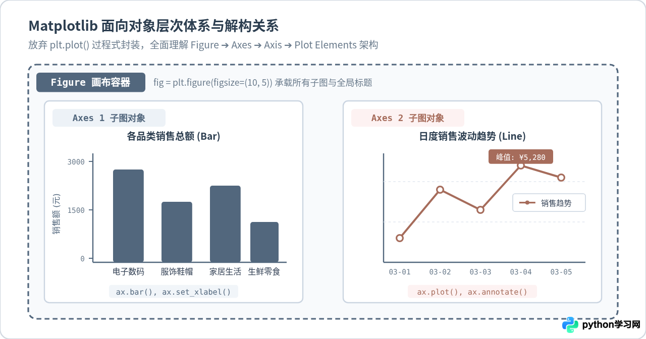
1. 解决中文显示方块与负号异常

Matplotlib 默认字体库不包含中文字形，若不显式指定，中文字符会全部渲染为白色空心方块（Tofu）。此外，Unicode 负号在某些字体下也会报错，需全局关闭 axes.unicode_minus：

import matplotlib.pyplot as plt

# 全局设置中文字体与负号正常显示
plt.rcParams['font.sans-serif'] = ['PingFang SC', 'Microsoft YaHei', 'SimHei', 'sans-serif']
plt.rcParams['axes.unicode_minus'] = False

2. 双子图协同绘制与美化设计

我们创建一个水平排列的双子图画布（1 行 2 列）：

左子图（ax1）：绘制品类销售总额的柱状图，并在柱子顶端动态标注具体金额标签；右侧次坐标轴叠加各品类订单件数折线，直观反映单价与件数的关系；
右子图（ax2）：绘制每日销售额走势折线图，添加数据节点标记（marker），标注销售峰值日期与金额；
细节修饰：统一配色为工程蓝灰 #52677D 与赭红 #A66C5B，去掉多余的顶部和右侧外边框（spines），增加浅灰色虚线网格，提升数据信噪比。

# 创建面向对象画布 (1行2列)
fig, (ax1, ax2) = plt.subplots(1, 2, figsize=(14, 5.5), dpi=100)

# ----------------- 左图：品类销售与数量双轴图 -----------------
colors = ['#52677D', '#647D96', '#7D95AD', '#9CB1C4']
bars = ax1.bar(
    category_summary['category'],
    category_summary['total_sales'],
    color=colors[:len(category_summary)],
    width=0.45,
    label='销售额 (元)'
)

# 柱顶数值标注
for bar in bars:
    height = bar.get_height()
    ax1.annotate(f'¥{height:,.0f}',
                 xy=(bar.get_x() + bar.get_width() / 2, height),
                 xytext=(0, 4), textcoords="offset points",
                 ha='center', va='bottom', fontsize=9.5, color='#2C3E50', fontweight='bold')

# 次坐标轴：总销售件数折线
ax1_twin = ax1.twinx()
ax1_twin.plot(category_summary['category'], category_summary['total_quantity'],
              color='#A66C5B', marker='o', linewidth=2, label='销售件数 (件)')

ax1.set_title('各商品品类销售额与件数对比', fontsize=13, fontweight='bold', pad=12, color='#2C3E50')
ax1.set_ylabel('销售总金额 (元)', fontsize=10.5, color='#52677D')
ax1_twin.set_ylabel('销售件数 (件)', fontsize=10.5, color='#A66C5B')
ax1.set_ylim(0, category_summary['total_sales'].max() * 1.2)
ax1_twin.set_ylim(0, category_summary['total_quantity'].max() * 1.4)

# 边框与网格微调
ax1.spines['top'].set_visible(False)
ax1_twin.spines['top'].set_visible(False)
ax1.grid(axis='y', linestyle='--', alpha=0.35)

# ----------------- 右图：日度销售走势图 -----------------
# 格式化日期显示为 MM-DD
date_labels = daily_trend['order_date'].dt.strftime('%m-%d')
ax2.plot(date_labels, daily_trend['daily_sales'],
         color='#52677D', linewidth=2.2, marker='s', markersize=6, markerfacecolor='#FFFFFF', markeredgewidth=2,
         label='日销售额')

# 标注最高销售峰值点
max_row = daily_trend.loc[daily_trend['daily_sales'].idxmax()]
max_date_str = max_row['order_date'].strftime('%m-%d')
max_val = max_row['daily_sales']

ax2.annotate(f'峰值: ¥{max_val:,.0f}',
             xy=(max_date_str, max_val),
             xytext=(0, 15), textcoords="offset points",
             ha='center', va='bottom',
             arrowprops=dict(arrowstyle='->', color='#A66C5B', lw=1.5),
             fontsize=10, fontweight='bold', color='#A66C5B',
             bbox=dict(boxstyle='round,pad=0.25', facecolor='#FDF2F2', edgecolor='#A66C5B', lw=0.8))

ax2.set_title('日度销售总额趋势走向', fontsize=13, fontweight='bold', pad=12, color='#2C3E50')
ax2.set_xlabel('日期 (月-日)', fontsize=10.5, color='#52677D')
ax2.set_ylabel('销售总额 (元)', fontsize=10.5, color='#52677D')
ax2.set_ylim(0, max_val * 1.25)
ax2.spines['top'].set_visible(False)
ax2.spines['right'].set_visible(False)
ax2.grid(axis='y', linestyle='--', alpha=0.35)
ax2.legend(loc='upper right', frameon=True)

# 保证布局紧凑，杜绝标签与图例裁切
fig.tight_layout()
plt.savefig('sales_analysis.png', dpi=150, bbox_inches='tight')
plt.show()

六、完整独立端到端运行代码

为了让读者能够直接验证上述所有逻辑，以下提供整合后的完整独立 Python 脚本。你可以直接将代码保存为 run_analysis.py 并在本地环境中执行：

import pandas as pd
import numpy as np
import matplotlib.pyplot as plt

def main():
    # 1. 构建模拟数据
    raw_data = {
        'order_id': [1001, 1002, 1002, 1003, 1004, 1005, 1006, 1007, 1008, 1009],
        'order_date': [
            '2024-03-01', '2024/03/02', '2024/03/02', '2024年03月03日', None,
            '2024-03-04', '2024-03-05', '2024-03-05', '2024-03-06', '2024-03-07'
        ],
        'unit_price': [
            '￥1,200.00', '450.0', '450.0', '￥89.50', '￥3,200.00',
            '120.0', '￥2,100.00', '78.0', '￥560.00', '￥1,100.00'
        ],
        'quantity': [2, 1, 1, -2, 1, 3, 2, 5, 0, 2],
        'category': ['电子数码', '服饰鞋帽', '服饰鞋帽', '生鲜食品', '家居生活', None, '电子数码', '生鲜食品', '家居生活', '电子数码']
    }
    df = pd.DataFrame(raw_data)

    # 2. 数据清洗流水线
    # (a) 标准化日期
    df['order_date'] = pd.to_datetime(
        df['order_date'].astype(str).str.replace('年', '-').str.replace('月', '-').str.replace('日', ''),
        errors='coerce'
    )
    # (b) 清洗数值列字符串
    df['unit_price'] = (
        df['unit_price'].str.replace('￥', '', regex=False).str.replace(',', '', regex=False).astype(float)
    )
    # (c) 主键去重与空值处置
    df = df.drop_duplicates(subset=['order_id'], keep='first')
    df = df.dropna(subset=['order_date'])
    df['category'] = df['category'].fillna('其他品类')
    
    # (d) 业务有效性过滤并拷贝副本
    clean_df = df[df['quantity'] > 0].copy()
    clean_df.reset_index(drop=True, inplace=True)
    clean_df['total_amount'] = clean_df['unit_price'] * clean_df['quantity']

    # 3. 分组聚合计算
    cat_summary = clean_df.groupby('category').agg(
        total_sales=('total_amount', 'sum'),
        total_quantity=('quantity', 'sum')
    ).reset_index().sort_values(by='total_sales', ascending=False)

    daily_trend = clean_df.groupby('order_date').agg(
        daily_sales=('total_amount', 'sum')
    ).reset_index().sort_values(by='order_date')

    # 4. Matplotlib 面向对象绘图
    plt.rcParams['font.sans-serif'] = ['PingFang SC', 'Microsoft YaHei', 'SimHei', 'sans-serif']
    plt.rcParams['axes.unicode_minus'] = False

    fig, (ax1, ax2) = plt.subplots(1, 2, figsize=(13, 5), dpi=120)

    # 左图：柱状图与次轴折线
    bars = ax1.bar(cat_summary['category'], cat_summary['total_sales'], color='#52677D', width=0.45)
    for b in bars:
        h = b.get_height()
        ax1.annotate(f'¥{h:,.0f}', xy=(b.get_x() + b.get_width() / 2, h),
                     xytext=(0, 3), textcoords="offset points", ha='center', fontsize=9)
    
    ax1_twin = ax1.twinx()
    ax1_twin.plot(cat_summary['category'], cat_summary['total_quantity'], color='#A66C5B', marker='o', lw=1.8)
    ax1.set_title('各品类销售额与订单销量', fontsize=12, fontweight='bold', color='#2C3E50')
    ax1.set_ylabel('销售额 (元)', color='#52677D')
    ax1_twin.set_ylabel('销售件数 (件)', color='#A66C5B')
    ax1.spines['top'].set_visible(False)
    ax1_twin.spines['top'].set_visible(False)
    ax1.grid(axis='y', ls='--', alpha=0.3)

    # 右图：日销售额走势
    date_strs = daily_trend['order_date'].dt.strftime('%m-%d')
    ax2.plot(date_strs, daily_trend['daily_sales'], color='#52677D', marker='s', lw=2, markerfacecolor='white')
    max_idx = daily_trend['daily_sales'].idxmax()
    ax2.annotate('销售峰值',
                 xy=(date_strs.iloc[max_idx], daily_trend['daily_sales'].iloc[max_idx]),
                 xytext=(0, 15), textcoords="offset points", ha='center',
                 arrowprops=dict(arrowstyle='->', color='#A66C5B', lw=1.2),
                 color='#A66C5B', fontweight='bold', fontsize=9.5)
    
    ax2.set_title('日度销售额走向趋势', fontsize=12, fontweight='bold', color='#2C3E50')
    ax2.set_ylabel('销售额 (元)', color='#52677D')
    ax2.spines['top'].set_visible(False)
    ax2.spines['right'].set_visible(False)
    ax2.grid(axis='y', ls='--', alpha=0.3)

    fig.tight_layout()
    plt.savefig('sales_analysis.png', dpi=150, bbox_inches='tight')
    print("可视化报表已保存为 sales_analysis.png")

if __name__ == '__main__':
    main()

七、数据分析全流程避坑总结

回顾从原始数据加载到最终图表落地的全过程，高效的数据分析并非单纯调用几个 API，而是要在每一个环节树立防御性编程意识。

关键结论备忘：

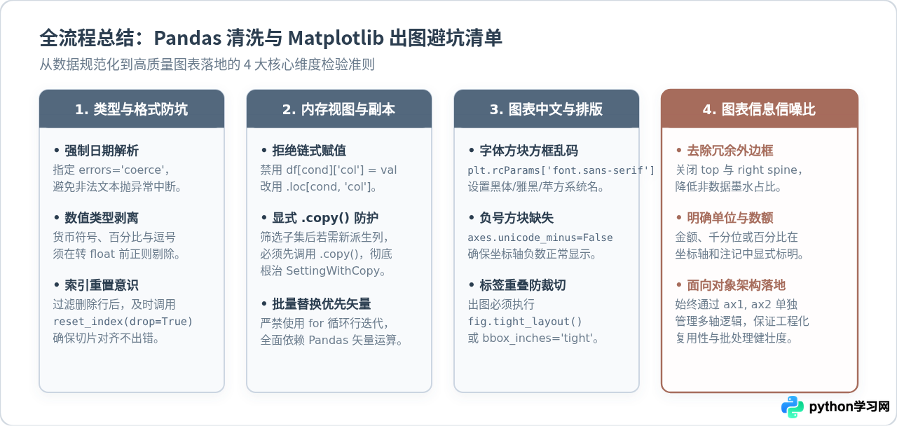
类型早定型：数据加载后的首要任务是把时间转为标准 datetime64、把金额转为 float。绝不要带着 object 类型的数值列进入下一步计算；
警惕切片警告：在对 DataFrame 进行行过滤时，务必养成后接 .copy() 的习惯，彻底切断底层数组视图的关联，避免触发臭名昭著的 SettingWithCopyWarning；
面向对象出图：尽量抛弃过程式的 plt.title()、plt.plot()，全面采用 fig, ax = plt.subplots() 搭配 ax.set_title() 等显式方法，保证图表组件层次分明、易于拓展和自动化批量产出。